In a previous ‘Math Matters’ blog post titled, “The Importance of Avoiding Large Losses,” we discussed the impacts of large losses on portfolios and wealth creation. Certainly, anyone who lived through the Dot-com crash of 2000-02 or the financial crisis of 2007-09 is well aware of the damage that losses of 30%, 40% or 50% can have on a portfolio.
What many people don’t know, however, is the impact that volatility drag has on the long-term success of an investment plan.
If bear markets can be described as a rare but catastrophic flood for a portfolio, then everyday volatility can be seen as water damage slowly that erodes away the foundations of your house (investment returns).

Source: Swan Global Investments
Investment returns are often stated as long-term averages. The problem with averages, however, is that averages mask details. The day-to-day or month-to-month experience of an investor might be radically different from the long-term averages. What happens in-between might have a large impact on the final wealth of an investor.
Again, we start with a simple illustration. If one were asked which of the following three scenarios would yield the best ten-year results, one might be tempted to choose the last of these three options:
Up 10% one year, down 5% the next, repeated for ten years
Up 25% one year, down 20% the next, repeated for ten years
Up 40% one year, down 35% the next, repeated for ten years
In fact, the opposite is true. After a decade:
Scenario A, with its most modest gains and losses, performs best and is the only scenario that is profitable;
Scenario B breaks even and;
Scenario C loses money.
This phenomenon is known as volatility drag. Also called variance drain, volatility drag was detailed in a 1995 paper by Tom Messmore titled “Variance Drain — Is your return leaking down the variance drain?”. Messmore observed that the more variable a given asset’s return is, the greater the difference between the arithmetic and geometric returns.
Arithmetic mean is the average of a set of numerical values, calculated by adding together and dividing by the number of terms in the set (Source: Wikipedia).
Geometric mean is defined as the value of a set of numbers by using the product of their values, as opposed to the arithmetic mean which uses their sum (Source: Wikipedia).

This formula shows that the variance of returns “drains” the arithmetic average returns to produce the smaller, realized, compound returns (Source: Decker, Robert: The Variance Drain and Jensen’s Inequality).
Why does this matter for investors?
It ties back to our previous posts on compounding returns and minimizing losses.
In order to optimally take advantage of the power of compounding, investors must avoid large losses and recoveries requiring exponential growth. In addition, investors must also avoid the negative power of compounding by seeking to lower volatility and variance drain as best as possible.
The table below shows different scenarios with the same arithmetic annual return (i.e. 10%) but coupled with different levels of volatility.
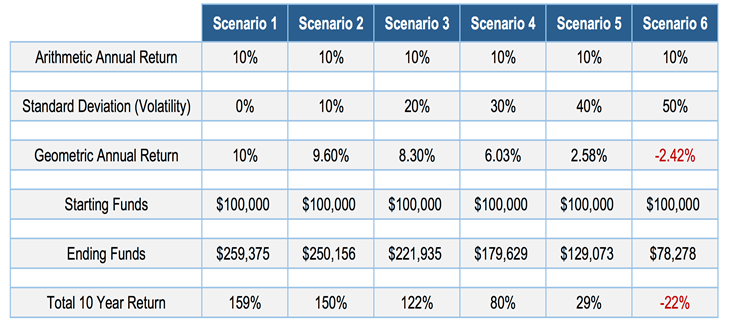
Source: Tyton Capital Advisors, “Low Charges And High Volatility: How To Erase Your Returns”
Generally speaking, there are two rules of thumb to remember when it comes to volatility drag.
The higher the level of volatility, the more detrimental the impact of volatility drag, as evidenced in the table above.
The longer the time period, the bigger the negative impact will be.
This situation is also explored in a post on volatility we wrote for ETFTrends.com. In addition, the greater the volatility, the more unlikely it is that an investor will be able to “stay the course” and stick with an investment or strategy.
We can see how these factors all tie together in their mathematical application within an investor’s portfolio: compounding, avoiding large losses, and now volatility. Compounding, whether negative or positive, is the common thread throughout all of them. As a recap, the four key mathematical principles outlined in “Math Matters” are:
The importance and power of compounding
The importance of variance drain
The value of a non-normal distribution of returns
The last post in this ‘Math Matters’ series will discuss changing the shape of distribution of returns.
Marc Odo, CFA®, CAIA®, CIPM®, CFP®, Client Portfolio Manager, is responsible for helping clients and prospects gain a detailed understanding of Swan’s Defined Risk Strategy, including how it fits into an overall investment strategy. Formerly Marc was the Director of Research for 11 years at Zephyr Associates.
Swan Global Investments, LLC is a SEC registered Investment Advisor that specializes in managing money using the proprietary Defined Risk Strategy (“DRS”). SEC registration does not denote any special training or qualification conferred by the SEC. Swan Global Investments offers and manages the Defined Risk Strategy for investors including individuals, institutions and other investment advisor firms. All Swan products utilize the Swan DRS but may vary by asset class, regulatory offering type, etc. Accordingly, all Swan DRS product offerings will have different performance results and comparing results among the Swan products and composites may be of limited use. Swan claims compliance with the Global Investment Performance Standards (GIPS®). Any historical numbers, awards and recognitions presented are based on the performance of a (GIPS®) composite, Swan’s DRS Select Composite, which includes nonqualified discretionary accounts invested in since inception, July 1997 and are net of fees and expenses. All data used herein; including the statistical information, verification and performance reports are available upon request. The S&P 500 Index is a market cap weighted index of 500 widely held stocks often used as a proxy for the overall U.S. equity market. Indexes are unmanaged and have no fees or expenses. An investment cannot be made directly in an index. Swan’s investments may consist of securities which vary significantly from those in the benchmark indexes listed above and performance calculation methods may not be entirely comparable. Accordingly, comparing results shown to those of such indexes may be of limited use. The adviser’s dependence on its DRS process and judgments about the attractiveness, value and potential appreciation of particular ETFs and options in which the adviser invests or writes may prove to be incorrect and may not produce the desired results. There is no guarantee any investment or the DRS will meet its objectives. All investments involve the risk of potential investment losses as well as the potential for investment gains. Prior performance is not a guarantee of future results and there can be no assurance, and investors should not assume, that future performance will be comparable to past performance. All investment strategies have the potential for profit or loss. Further information is available upon request by contacting the company directly at 970.382.8901 or visit www.swanglobalinvestments.com. 245-SGI-092716